
We propose to implement a simple Artificial Neural Network (ANN) from scratch using only the Numpy library. Although it is more efficient to use deep learning libraries such as Tensorflow or Pytorch, the motivation is to have a better understanding of how ANNs work.
Architecture
We will look at implementing an ANN with 3 input neurons. This means that our problem has 3 features and 1 binary output variable. The architecture is shown below.
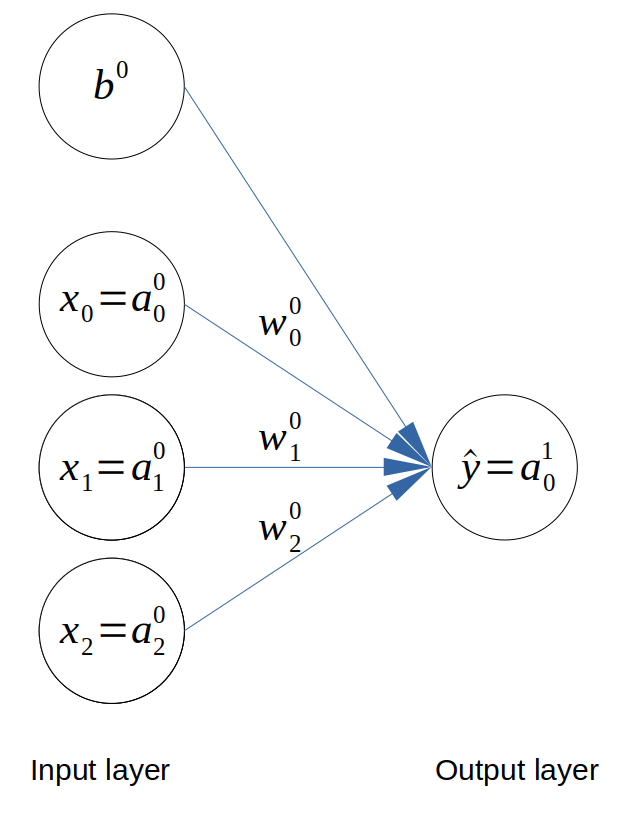 Architecture of the neural network
For each variable, the layer number is shown in superscript and the item number in each variable is shown in subscript. For example, \(w^L_i\) is the \(i^{th}\) weight in layer \(L\).
Feedforward
We will derive the equations as in the previous posts. Please refer to them for more details. The activation of the predicted output \(\hat{y}\) can be written as follows,
\[\hat{y} = a^1_0 = \sigma(z^1_0)\]From the network architecture, we get:
\[z^1_0 = a^0_0 w^0_0 + a^0_1 w^0_1 + a^0_2 w^0_2 + b^0\]Backpropagation
The MSE cost function is defined as follows,
\[J = \frac{1}{m}\sum_{i=1}^{m}(a^1_{0i}-y_i)^2\]Let’s apply Gradient Descent to the first weight \(w^0_0\).
\[w^0_0 := w^0_0 - \alpha \frac{\partial J}{\partial w^0_0}\]The chain rule now becomes,
\[\frac{\partial J}{\partial w^0_0} = \frac{\partial J}{\partial a^1_0} \frac{\partial a^1_0}{\partial z^1_0} \frac{\partial z^1_0}{\partial w^0_0}\]Isolating each terms, we have:
\[\begin{align*} \frac{\partial J}{\partial a^1_0} &= \frac{2}{m}(a^1_0-y) \\ \frac{\partial a^1_0}{\partial z^1_0} &= \sigma'(z^1_0) \\ \frac{\partial z^1_0}{\partial w^0_0} &= a^0_0 \end{align*}\]If we repeat the same steps for the other 2 weights and the bias, we get:
\[\begin{align*} \frac{\partial J}{\partial w^0_0} &= \frac{2}{m}(a^1_0-y) \sigma'(z^1_0) a^0_0 \\ \frac{\partial J}{\partial w^0_1} &= \frac{2}{m}(a^1_0-y) \sigma'(z^1_0) a^0_1 \\ \frac{\partial J}{\partial w^0_2} &= \frac{2}{m}(a^1_0-y) \sigma'(z^1_0) a^0_2 \\ \frac{\partial J}{\partial b^0} &= \frac{2}{m}(a^1_0-y) \sigma'(z^1_0) \end{align*}\]We are now ready to implement!
Numpy implementation
The implementation is inspired from this article.
The problem
efore tackling the implementation itself, we need to define a problem to solve. Let’s build a toy dataset for a simple classification problem. Suppose we have some information about obesity, smoking habits, and exercise habits of five people. We also know whether these people are diabetic or not. We can encode this information as follows:
| Person | Smoking | Obesity | Exercise | Diabetic |
|---|---|---|---|---|
| Person 1 | 0 | 1 | 0 | 1 |
| Person 2 | 0 | 0 | 1 | 0 |
| Person 3 | 1 | 0 | 0 | 0 |
| Person 4 | 1 | 1 | 0 | 1 |
| Person 5 | 1 | 1 | 1 | 1 |
In the above table, we have five columns (i.e. 5 observations): Person, Smoking, Obesity, Exercise, and Diabetic. Here 1 refers to true and 0 refers to false. For instance, the first person has values of 0, 1, 0 which means that the person doesn’t smoke, is obese, and doesn’t exercise. The person is also diabetic.
It is clearly evident from the dataset that a person’s obesity is indicative of him being diabetic. Our task is to create a neural network that is able to predict whether an unknown person is diabetic or not given data about his exercise habits, obesity, and smoking habits. This is a type of supervised learning problem where we are given inputs and corresponding correct outputs and our task is to find the mapping between the inputs and the outputs.
The code
We will base our implementation on the neural network architecture described above. We start by importing some libraries and defining the Sigmoid function and its derivative.
from matplotlib import pyplot as plt
import numpy as np


def sigmoid(x):
    return 1/(1+np.exp(-x))

def sigmoid_der(x):
    return sigmoid(x) * (1-sigmoid(x))
We then define our data set based on the problem described above.
X = np.array([[0, 1, 0], [0, 0, 1], [1, 0, 0], [1, 1, 0], [1, 1, 1]])
y = np.array([[1, 0, 0, 1, 1]])
y = y.reshape(5, 1)
We initialise the weights and biases randomly and we define the hyperparameters of the model.
np.random.seed(42)
weights = np.random.rand(3, 1)
bias = np.random.rand(1)
alpha = 0.05        # learning rate
nb_epoch = 20000
H = np.zeros((nb_epoch, 6))  # history
m = len(X)   # number of observations
During the training phase, we perform feedforward and backpropagation steps using the MSE cost function, the chain rule and the gradient descent algorithm.
for epoch in range(nb_epoch):

    # FEEDFORWARD
    z = np.dot(X, weights) + bias  # (5x1)
    a = sigmoid(z)  # (5X1)

    # BACKPROPAGATION
    # 1. cost function: MSE
    J = (1/m) * (a - y)**2   # (5X1)

    # 2. weights
    dJ_da = (2/m)*(a-y)
    da_dz = sigmoid_der(z)
    dz_dw = X.T

    gradient_w = np.dot(dz_dw, da_dz*dJ_da)  # chain rule
    weights -= alpha*gradient_w               # gradient descent

    # 3. bias
    gradient_b = da_dz*dJ_da   # chain rule
    bias -= alpha*sum(gradient_b)  # gradient descent

    # Record history for plotting
    H[epoch, 0] = epoch
    H[epoch, 1] = J.sum()
    H[epoch, 2:5] = np.ravel(weights)
    H[epoch, 5] = np.asscalar(bias)

    print("Epoch {}/{} | cost function: {}".format(epoch, nb_epoch, J.sum()))
We can then plot the evolution of the cost function, weights and bias with the number of iterations (epoch).
plt.plot(H[:, 0], H[:, 1])
plt.xlabel('Epoch #')
plt.ylabel('Training error')
plt.savefig('plots/1_J_vs_epoch.png')
plt.show()

plt.plot(H[:, 0], H[:, 2], label='$w_{11}$')
plt.plot(H[:, 0], H[:, 3], label='$w_{21}$')
plt.plot(H[:, 0], H[:, 4], label='$w_{31}$')
plt.xlabel('Epoch #')
plt.ylabel('Weights')
plt.legend()
plt.savefig('plots/1_weights_vs_epoch.png')
plt.show()

plt.plot(H[:, 0], H[:, 5])
plt.xlabel('Epoch #')
plt.ylabel('Bias')
plt.savefig('plots/1_bias_vs_epoch.png')
plt.show()
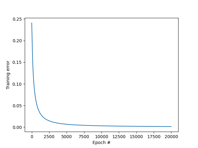 MSE vs epoch
The training error (MSE) keeps decreasing with the number of iterations, which is a good sign.
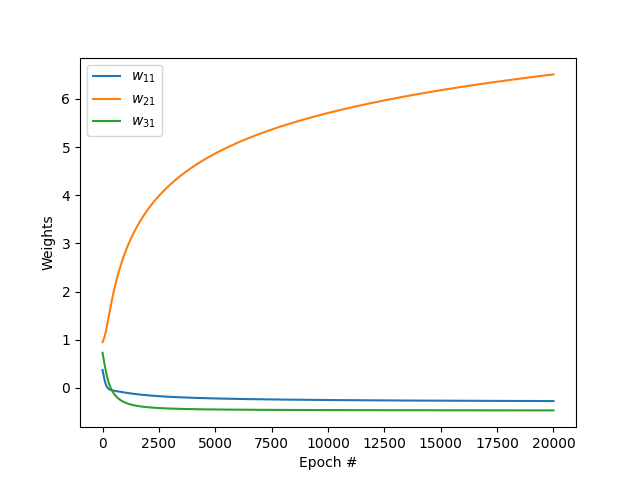 Weights vs epoch
We can also notice that the weight \(w_{21}\) becomes predominant after many iterations. This is because the 2nd feature (obesity) is very highly correlated with the output variable (diabetic).
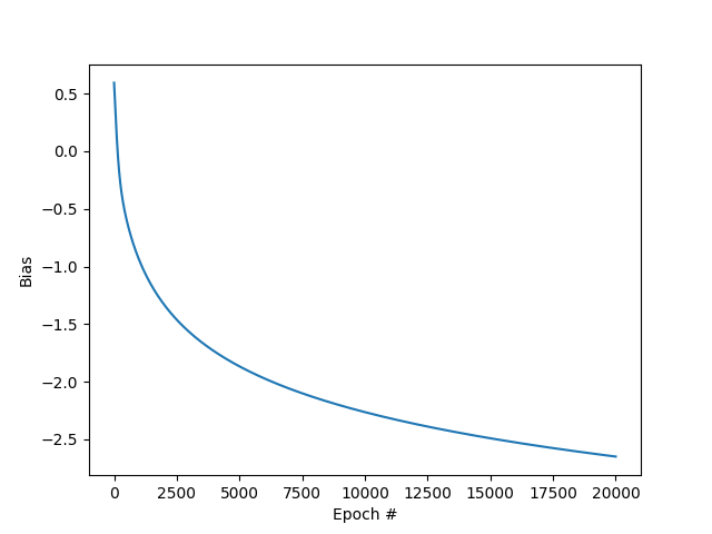 Bias vs epoch
Finally, we test our neural network on some unseen examples. Let’s consider two “new” people who did not appear in the training set. For example, a smoker not obese who does some exercise (defined by [1, 0, 1]) is classified as not diabetic.
example1 = np.array([1, 0, 1])
result1 = sigmoid(np.dot(example1, weights) + bias)
print(result1.round())

>> [0.]
However, an obese non-smoker who exercises ([0, 1, 1]) is predicted to be diabetic.
example2 = np.array([0, 1, 1])
result2 = sigmoid(np.dot(example2, weights) + bias)
print(result2.round())

>> [1.]
You can find the code on my Github.
Conclusion
This article described the theory of a very simple neural network with one input layer and one output layer. It was implemented in plain Numpy and applied to a simple classification problem with 3 features and 5 observations.
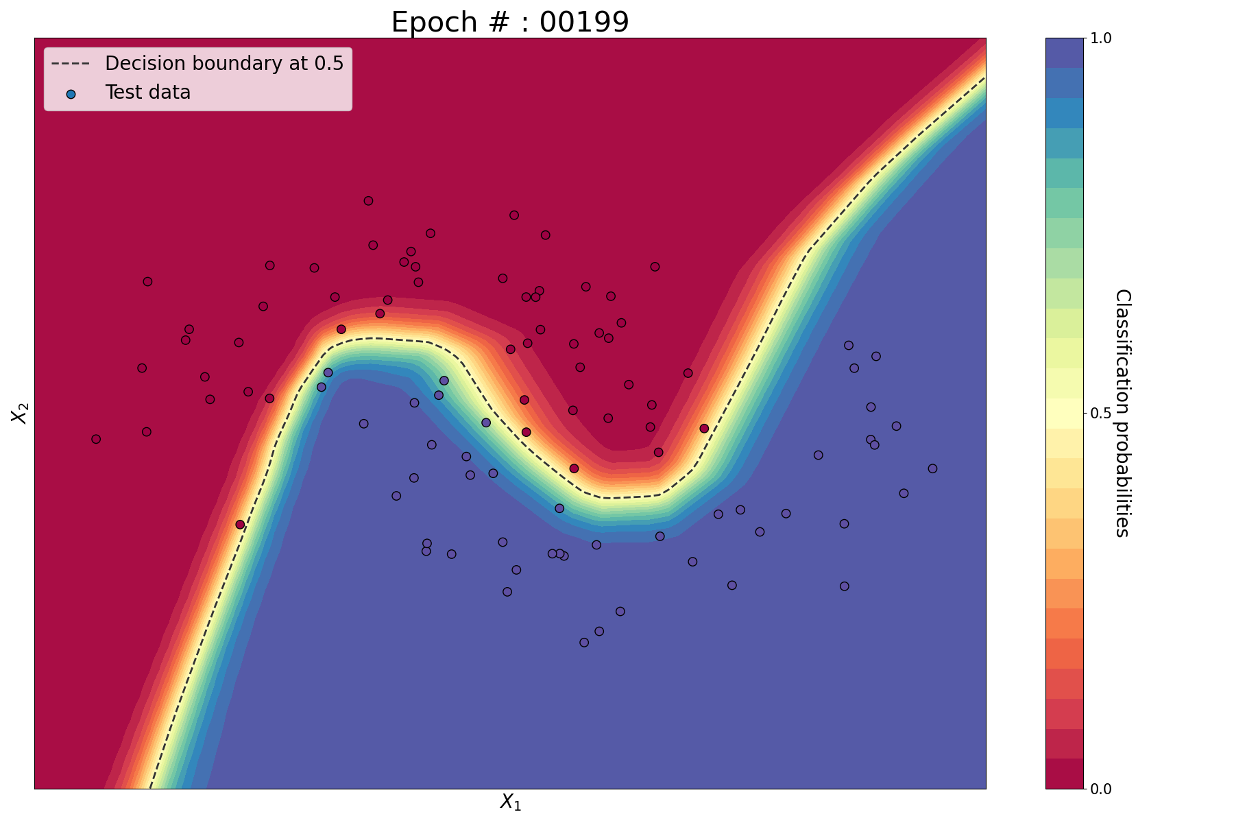
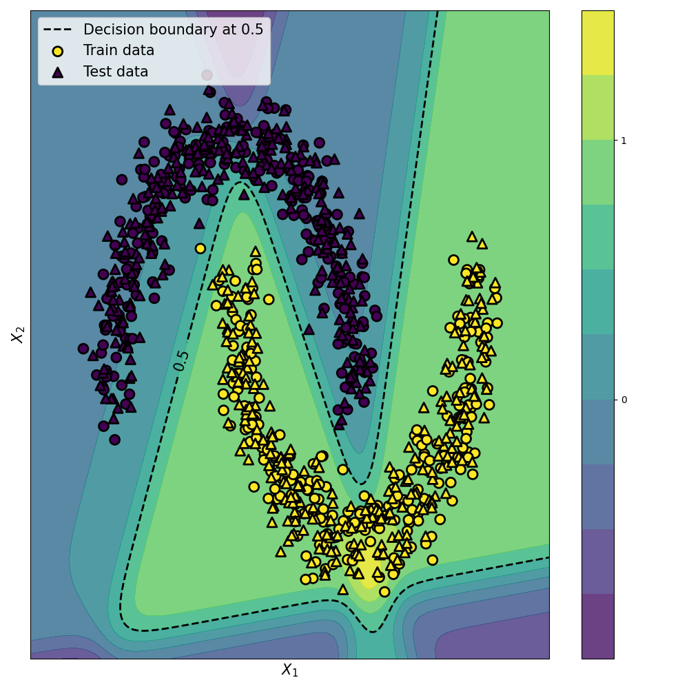
This type of neural network is called a Single-Layer Perceptron and it is capable of classify linearly separable data. However, most real-world problems require to identify non-linear decision boundaries. In the next article, I will describe how Multi-Layer Perceptron can be used to estimate non-linear decision boundaries.


Leave a comment